The gender gap in household work narrowed more among married adults

Average daily minutes of household activities reported by U.S. adults ages 25–64

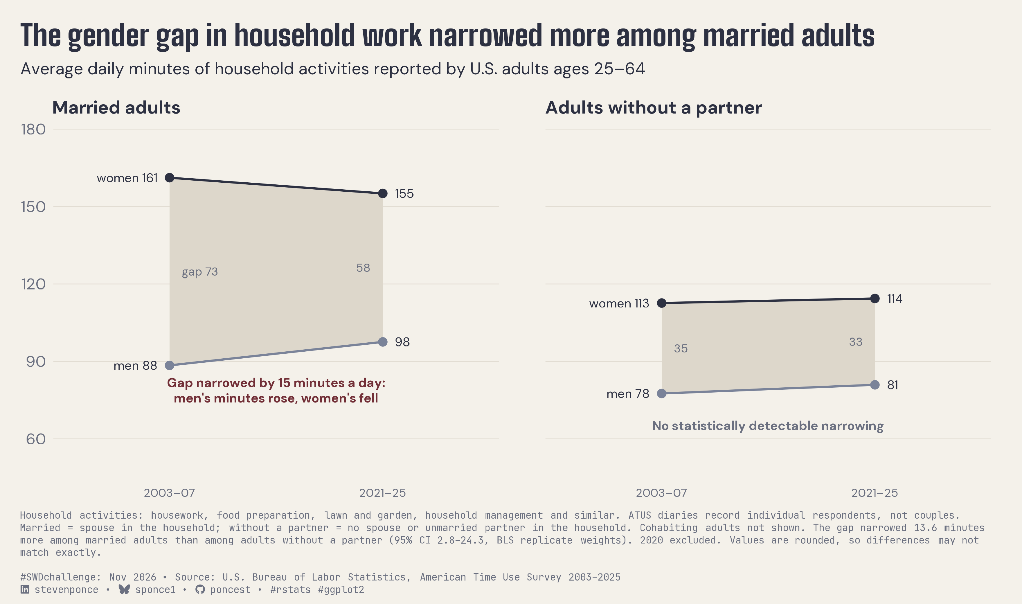
Gap ribbons show the gender gap in daily household-activity minutes narrowing by 15 minutes among married U.S. adults between 2003–07 and 2021–25, with no statistically detectable narrowing among adults without a partner. Weighted ATUS means, with the difference in changes tested using BLS replicate weights. Built in R with ggplot2, ggtext, and showtext.

Challenge

Change is constant—in life and in data. This month, your challenge is to create a visualization that helps your audience see what changed and why it matters. This month, we’re focusing on change. Whether you explore a dramatic shift or a subtle evolution, your task is to help your audience understand what’s different and why it deserves their attention.

Additional information can be found HERE

Visualization

Figure 1: Two-panel gap-ribbon chart titled “The gender gap in household work narrowed more among married adults.” Among married U.S. adults ages 25–64, the gap between women’s and men’s average daily household-activity minutes narrowed from 73 to 58, a 15-minute reduction, as men’s minutes rose from 88 to 98 and women’s fell from 161 to 155. Among adults without a spouse or unmarried partner in the household, the gap fell from 35 to 33 minutes (women 113 to 114, men 78 to 81), a change not statistically detectable. Each panel compares 2003–07 with 2021–25 on the same vertical scale, with a shaded band between the women’s and men’s lines marking the gap. The two groups’ changes differed by 13.6 minutes a day (95% CI 2.8–24.3). Data: U.S. Bureau of Labor Statistics, American Time Use Survey; individual respondents, not couples; 2020 excluded.

Reproducibility

This page contains the R code used to generate the descriptive visualization.

Data: Download the ATUS 2003–2025 Activity Summary file from the U.S. Bureau of Labor Statistics and extract atussum_0325.dat to data/SWDchallenge/2026/ in the personal-website repository.

The chart uses the ATUS final survey weight (TUFNWGTP). The reported 95% confidence interval was calculated separately using the 160 official BLS replicate weights.

The statistical decision record is intended to reproduce that inferential analysis and requires the additional replicate-weights file, atuswgts_0325.dat.

The raw data files are not committed to GitHub because of their size. Reproduction also requires the custom plotting utilities and font setup included in this repository.

The published website uses Quarto’s frozen execution and caching. To verify the calculations independently, rerun the analysis rather than relying on previously generated output.

Steps to Create this Graphic

1. Load Packages & Setup

```{r}
#| label: load

if (!require("pacman")) install.packages("pacman")
pacman::p_load(
  tidyverse, ggtext, showtext, janitor, scales, glue, ggview
  )

# Source utility functions
suppressMessages(source(here::here("R/utils/fonts.R")))
source(here::here("R/utils/social_icons.R"))
source(here::here("R/utils/image_utils.R"))
source(here::here("R/themes/base_theme.R"))

### |- figure settings ----
fig_w   <- 11
fig_h   <- 6.5
fig_dpi <- 320

### |- fonts ----
setup_fonts()
fonts <- get_font_families()
title_family <- fonts$title_1
text_family  <- fonts$text
caption_family  <- fonts$caption
```

2. Read in the Data

```{r}
#| label: read

data_path <- here::here("data/SWDchallenge/2026/atussum_0325.dat")

atus_raw <- read_csv(
  data_path,
  col_select = c(TUCASEID, TESEX, TEAGE, TRSPPRES, TUYEAR, TUFNWGTP, starts_with("t02")),
  col_types = cols(TUCASEID = col_character(), .default = col_double())
)
```

3. Examine the Data

```{r}
#| label: examine
#| include: true
#| eval: true
#| results: 'hide'
#| warning: false

glimpse(atus_raw |> select(TUCASEID:TUFNWGTP))
atus_raw |> count(TUYEAR)
atus_raw |> count(TRSPPRES)
```

4. Tidy Data

```{r}
#| label: tidy
#| output: false

### |- analysis frame: ages 25-64, 2020 excluded, two pooled periods ----
hh_df <- atus_raw |>
  mutate(hh_min = rowSums(pick(starts_with("t02")))) |>
  filter(between(TEAGE, 25, 64), TUYEAR != 2020) |>
  mutate(
    period = case_when(
      between(TUYEAR, 2003, 2007) ~ "2003–07",
      between(TUYEAR, 2021, 2025) ~ "2021–25"
    ),
    group = case_match(TRSPPRES, 1 ~ "Married adults", 3 ~ "Adults without a partner"),
    sex = if_else(TESEX == 2, "women", "men")
  ) |>
  filter(!is.na(period), !is.na(group))

### |- weighted means by group x period x sex ----
ribbon_df <- hh_df |>
  summarise(minutes = weighted.mean(hh_min, TUFNWGTP), n = n(), .by = c(group, period, sex)) |>
  mutate(
    group = factor(group, levels = c("Married adults", "Adults without a partner")),
    x = if_else(period == "2003–07", 1, 2)
  )

gap_df <- ribbon_df |>
  select(group, period, x, sex, minutes) |>
  pivot_wider(names_from = sex, values_from = minutes) |>
  mutate(gap = women - men)

get_val <- function(g, p, col) {
  gap_df |>
    filter(group == g, period == p) |>
    pull({{ col }})
}
m_gap_1 <- get_val("Married adults", "2003–07", gap)
m_gap_2 <- get_val("Married adults", "2021–25", gap)
n_gap_1 <- get_val("Adults without a partner", "2003–07", gap)
n_gap_2 <- get_val("Adults without a partner", "2021–25", gap)
m_men_chg <- get_val("Married adults", "2021–25", men) - get_val("Married adults", "2003–07", men)
m_women_chg <- get_val("Married adults", "2021–25", women) - get_val("Married adults", "2003–07", women)
diff_in_changes <- (n_gap_2 - n_gap_1) - (m_gap_2 - m_gap_1)

# Validated using the official BLS replicate-weight analysis.
# This script reproduces the descriptive chart, not the CI.
# Retain the separate statistical decision record for full replication.
did_ci <- c(lo = 2.8, hi = 24.3)
```

5. Visualization Parameters

```{r}
#| label: params

### |- plot aesthetics ----
colors <- get_theme_colors(
  palette = list(
    women = "#2D3142",
    men = "#7A8399",
    band = "#DDD7CB",
    accent = "#722F37",
    soft = "#6B7080",
    paper = "#F4F1EA"
  )
)
clrs <- colors$palette
fallback <- c(
  women = "#2D3142", men = "#7A8399", band = "#DDD7CB", accent = "#722F37",
  soft = "#6B7080", paper = "#F4F1EA"
)
for (k in names(fallback)) if (is.null(clrs[[k]])) clrs[[k]] <- fallback[[k]]

### |- titles and caption ----
title_text <- "The gender gap in household work narrowed more among married adults"

subtitle_text <- "Average daily minutes of household activities reported by U.S. adults ages 25–64"

note_text <- glue(
  "Household activities: housework, food preparation, lawn and garden, household management and similar. ",
  "ATUS diaries record individual respondents, not couples. Married = spouse in the household; without a partner = ",
  "no spouse or unmarried partner in the household. Cohabiting adults not shown. The gap narrowed {round(diff_in_changes, 1)} ",
  "minutes more among married adults than among adults without a partner (95% CI {did_ci[['lo']]}–{did_ci[['hi']]}, BLS replicate weights). 2020 excluded. ",
  "Values are rounded, so differences may not match exactly.<br>"
)

caption_text <- paste0(
  note_text, "<br>",
  create_swd_caption(
    year = 2026,
    month = "Nov",
    source_text = "U.S. Bureau of Labor Statistics, American Time Use Survey 2003–2025"
  )
)

ann_df <- tibble(
  group = factor(c("Married adults", "Adults without a partner"), levels = levels(ribbon_df$group)),
  label = c(
    glue("Gap narrowed by {round(m_gap_1 - m_gap_2)} minutes a day:\nmen's minutes rose, women's fell"),
    "No statistically detectable narrowing"
  ),
  colour = c(clrs$accent, clrs$soft)
) |>
  left_join(gap_df |> filter(x == 2) |> select(group, men), by = "group") |>
  mutate(y = men - 14)

### |- in-band gap labels ("gap" named once: married panel, 2003-07 side) ----
gap_lab <- gap_df |>
  mutate(
    y = (women + men) / 2,
    label = if_else(group == "Married adults" & x == 1,
      as.character(glue("gap {round(gap)}")), as.character(round(gap))
    ),
    hjust = if_else(x == 1, 0, 1),
    x = if_else(x == 1, x + 0.06, x - 0.06)
  )

end_labels <- ribbon_df |>
  mutate(label = if_else(x == 1, as.character(glue("{sex} {round(minutes)}")), as.character(round(minutes))))

### |- plot theme ----
base_theme <- create_base_theme(colors)

weekly_theme <- extend_weekly_theme(
  base_theme,
  theme(
    plot.background = element_rect(fill = clrs$paper, colour = NA),
    panel.background = element_rect(fill = clrs$paper, colour = NA),
    plot.title = element_text(
      family = title_family, size = rel(1.6), colour = clrs$women,
      margin = margin(b = 8)
    ),
    plot.subtitle = element_text(
      family = text_family, size = rel(0.92), colour = clrs$women,
      lineheight = 1.2, margin = margin(b = 16)
    ),
    plot.caption = element_textbox_simple(
      family = caption_family, size = rel(0.55), colour = clrs$soft,
      lineheight = 1.25, width = unit(1, "npc"), halign = 0,
      margin = margin(t = 14)
    ),
    plot.title.position = "plot", plot.caption.position = "plot",
    strip.text = element_text(
      family = text_family, face = "bold", size = rel(1.0), colour = clrs$women,
      hjust = 0, margin = margin(b = 8)
    ),
    axis.title.x = element_blank(),
    axis.title.y = element_blank(),
    axis.text = element_text(family = text_family, colour = clrs$soft, size = rel(0.85)),
    axis.text.x = element_text(family = text_family, colour = clrs$soft, size = rel(0.75)),
    axis.ticks = element_blank(),
    panel.grid.minor = element_blank(), panel.grid.major.x = element_blank(),
    panel.grid.major.y = element_line(colour = "#E2DDD3", linewidth = 0.3),
    panel.spacing = unit(2.5, "lines"),
    plot.margin = margin(18, 24, 12, 16)
  )
)
theme_set(weekly_theme)
```

6. Plot

```{r}
#| label: plot
#| output: false

### |-  plot ----
p <- ggplot() +
  # Geoms
  geom_ribbon(data = gap_df, aes(x = x, ymin = men, ymax = women), fill = clrs$band) +
  geom_text(
    data = gap_lab, aes(x, y, label = label, hjust = hjust),
    family = text_family, size = 3.2, colour = clrs$soft
  ) +
  geom_line(data = ribbon_df, aes(x, minutes, group = sex, colour = sex), linewidth = 0.8) +
  geom_point(data = ribbon_df, aes(x, minutes, colour = sex), size = 2.6) +
  geom_text(
    data = filter(end_labels, x == 1), aes(x - 0.06, minutes, label = label),
    hjust = 1, family = text_family, size = 3.4, colour = clrs$women
  ) +
  geom_text(
    data = filter(end_labels, x == 2), aes(x + 0.06, minutes, label = label),
    hjust = 0, family = text_family, size = 3.4, colour = clrs$women
  ) +
  # Annotations
  geom_text(
    data = ann_df[1, ], aes(x = 1.5, y = y, label = label), colour = clrs$accent,
    family = text_family, size = 3.5, fontface = "bold", lineheight = 1.0, vjust = 1
  ) +
  geom_text(
    data = ann_df[2, ], aes(x = 1.5, y = y, label = label), colour = clrs$soft,
    family = text_family, size = 3.5, fontface = "bold", lineheight = 1.0, vjust = 1
  ) +
  # Scales
  scale_colour_manual(values = c(men = clrs$men, women = clrs$women), guide = "none") +
  scale_x_continuous(breaks = 1:2, labels = c("2003–07", "2021–25"), limits = c(0.55, 2.45)) +
  scale_y_continuous(breaks = seq(60, 180, 30)) +
  coord_cartesian(ylim = c(50, 175), clip = "off") +
  facet_wrap(~group) +
  # Labs
  labs(title = title_text, subtitle = subtitle_text, caption = caption_text, y = NULL)
```

7. Save

```{r}
#| label: save
#| warning: false

### |- save ----
main_path  <- here::here("data_visualizations", "SWD Challenge", "2026", "swd_2026_11.png")
thumb_path <- here::here("data_visualizations", "SWD Challenge", "2026", "thumbnails", "swd_2026_11.png")

# Full-size version, for the QMD figure
save_ggplot(
  plot = p,
  file = main_path,
  width = fig_w,
  height = fig_h,
  units = "in",
  dpi = fig_dpi,
  create.dir = TRUE
)

# Reduced-size thumbnail, for the YAML `image:` field
fs::dir_create(dirname(thumb_path))
magick::image_read(main_path) |>
  magick::image_resize("400") |>
  magick::image_write(thumb_path)
```

8. Session Info

TipExpand for Session Info

R version 4.6.1 (2026-06-24)
Platform: aarch64-apple-darwin23
Running under: macOS Tahoe 26.6.2

Matrix products: default
BLAS:   /Library/Frameworks/R.framework/Versions/4.6/Resources/lib/libRblas.0.dylib 
LAPACK: /Library/Frameworks/R.framework/Versions/4.6/Resources/lib/libRlapack.dylib;  LAPACK version 3.12.1

locale:
[1] en_US.UTF-8/en_US.UTF-8/en_US.UTF-8/C/en_US.UTF-8/en_US.UTF-8

time zone: America/New_York
tzcode source: internal

attached base packages:
[1] stats     graphics  grDevices utils     datasets  methods   base     

other attached packages:
 [1] here_1.0.2      ggview_0.2.2    glue_1.8.1      scales_1.4.0   
 [5] janitor_2.2.1   showtext_0.9-8  showtextdb_3.0  sysfonts_0.8.9 
 [9] ggtext_0.2.0    lubridate_1.9.5 forcats_1.0.1   stringr_1.6.0  
[13] dplyr_1.2.1     purrr_1.2.2     readr_2.2.0     tidyr_1.3.2    
[17] tibble_3.3.1    ggplot2_4.0.3   tidyverse_2.0.0 pacman_0.5.1   

loaded via a namespace (and not attached):
 [1] gtable_0.3.6       xfun_0.60          htmlwidgets_1.6.4  tzdb_0.5.0        
 [5] vctrs_0.7.3        tools_4.6.1        generics_0.1.4     curl_7.1.0        
 [9] parallel_4.6.1     pkgconfig_2.0.3    RColorBrewer_1.1-3 S7_0.2.2          
[13] lifecycle_1.0.5    compiler_4.6.1     farver_2.1.2       textshaping_1.0.5 
[17] codetools_0.2-20   snakecase_0.11.1   litedown_0.10      htmltools_0.5.9   
[21] yaml_2.3.12        pillar_1.11.1      crayon_1.5.3       magick_2.9.1      
[25] commonmark_2.0.0   tidyselect_1.2.1   digest_0.6.39      stringi_1.8.7     
[29] rprojroot_2.1.1    fastmap_1.2.0      grid_4.6.1         cli_3.6.6         
[33] magrittr_2.0.5     withr_3.0.3        bit64_4.8.2        timechange_0.4.0  
[37] rmarkdown_2.31     bit_4.6.0          otel_0.2.0         ragg_1.5.2        
[41] hms_1.1.4          evaluate_1.0.5     knitr_1.51         markdown_2.0      
[45] rlang_1.3.0        gridtext_0.1.6     Rcpp_1.1.2         xml2_1.6.0        
[49] rstudioapi_0.19.0  vroom_1.7.1        jsonlite_2.0.0     R6_2.6.1          
[53] fs_2.1.0           systemfonts_1.3.2 

9. GitHub Repository

TipExpand for GitHub Repo

The complete code for this analysis is available in swd_2026_11.qmd. For the full repository, click here.

10. References

TipExpand for References

SWD Challenge: - Storytelling with Data: November 2026 — tell a story of change

Data Sources: - U.S. Bureau of Labor Statistics. American Time Use Survey (ATUS) 2003–2025 Multi-Year Microdata Files. https://www.bls.gov/tus/data/datafiles-0325.htm - Activity Summary file (atussum_0325.dat): total minutes each respondent spent on each activity on their diary day. The chart’s outcome is the sum of the 32 household-activity codes (t02*), with means weighted by TUFNWGTP. - Replicate Weights file (atuswgts_0325.dat): 160 replicate weights, used only to compute confidence intervals. These do not appear on the chart, apart from the CI in the caption. - U.S. Bureau of Labor Statistics. ATUS 2003–2025 Coding Lexicon. https://www.bls.gov/tus/lexicons/lexiconnoex0325.pdf: the definitions of the household-activity (t02) codes. - U.S. Bureau of Labor Statistics. American Time Use Survey User’s Guide. https://www.bls.gov/tus/atususersguide.pdf: the successive-difference replication variance method, Var = 4/160 × Σ(θᵣ − θ₀)².

Analysis Frame: - Ages 25–64. The two periods are 2003–07 and 2021–25, and 2020 is excluded. - Groups come from TRSPPRES: 1 = spouse present (married); 3 = no spouse or unmarried partner in the household. Cohabiting adults (2) are left out of the chart. - The data are individual respondents, not matched couples. The comparison is descriptive, not causal.

Data Preparation: - Decision record: swd_2026_11_decision_record.R. It recomputes the difference in gap changes between the groups (13.6 minutes, 95% CI 2.8–24.3) and the component changes, using BLS replicate weights. It is kept separate from the chart script. - The raw .dat files are not in the repository. Download them from the BLS link above.

11. Custom Functions Documentation

Note📦 Custom Helper Functions

This analysis uses custom functions from my personal module library for efficiency and consistency across projects.

Functions Used:

• fonts.R: setup_fonts(), get_font_families() - Font management with showtext
• social_icons.R: create_swd_caption() - Generates the SWD caption with source and social handles
• base_theme.R: create_base_theme(), extend_weekly_theme(), get_theme_colors() - Custom ggplot2 themes

Why custom functions?
These utilities standardize theming, fonts, and output across all my data visualizations. The core analysis (data tidying and visualization logic) uses only standard tidyverse packages.

Source Code:
View all custom functions → GitHub: R/utils